Introduction
TileDB-SOMA is a cloud-native, array-based format for single-cell data. It is the storage backend behind CELLxGENE Census, which hosts 61M+ cells across 900+ datasets. SOMA supports efficient slicing by cells or features without loading the full dataset, making it ideal for working with large atlases.
scConvert provides writeSOMA() and
readSOMA() for Seurat interoperability. Both functions
require the tiledbsoma R
package. SOMA experiments are database-like stores rather than single
files, so they cannot easily be shipped as package demo data. Instead,
we start from the shipped RDS and demonstrate the round-trip.
Load demo data
We use a 500-cell PBMC dataset that ships with scConvert. It has 9 annotated cell types, PCA/UMAP embeddings, and neighbor graphs.
pbmc <- readRDS(system.file("extdata", "pbmc_demo.rds", package = "scConvert"))
pbmc
#> An object of class Seurat
#> 2000 features across 500 samples within 1 assay
#> Active assay: RNA (2000 features, 2000 variable features)
#>  2 layers present: counts, data
#>  2 dimensional reductions calculated: pca, umap
DimPlot(pbmc, reduction = "umap", group.by = "seurat_annotations",
        label = TRUE, pt.size = 0.8) +
  ggtitle("PBMC demo -- 9 cell types") + NoLegend()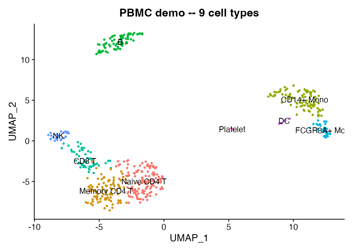
Write to SOMA
Save the Seurat object as a SOMA experiment. If tiledbsoma is not installed, this section shows the code without running it.
soma_uri <- file.path(tempdir(), "pbmc_demo.soma")

# Ensure graphs have a valid DefaultAssay (required by tiledbsoma)
for (gn in names(pbmc@graphs)) {
  if (length(DefaultAssay(pbmc@graphs[[gn]])) == 0) {
    DefaultAssay(pbmc@graphs[[gn]]) <- DefaultAssay(pbmc)
  }
}

writeSOMA(pbmc, uri = soma_uri, overwrite = TRUE)
cat("SOMA experiment written to:", soma_uri, "\n")Compare original and round-trip
Side-by-side UMAP plots confirm that cluster labels and coordinates survive the SOMA round-trip.
library(patchwork)

p1 <- DimPlot(pbmc, reduction = "umap", group.by = "seurat_annotations",
              label = TRUE, pt.size = 0.8) +
  ggtitle("Original") + NoLegend()

p2 <- DimPlot(pbmc_rt, reduction = "umap", group.by = "seurat_annotations",
              label = TRUE, pt.size = 0.8) +
  ggtitle("After SOMA round-trip") + NoLegend()

p1 + p2CELLxGENE Census access
CELLxGENE Census stores the largest public atlas of single-cell data
as a single SOMA experiment. You can query it with
readSOMA() and then convert the result to any format.
library(cellxgene.census)

census <- open_soma(census_version = "stable")
human_uri <- census$get("census_data")$get("homo_sapiens")$uri

# Read a subset directly as a Seurat object
tcells <- readSOMA(
  uri = human_uri,
  measurement = "RNA",
  obs_query = "cell_type == 'T cell' & tissue_general == 'blood'"
)

# Save locally in any format
writeH5AD(tcells, "census_tcells.h5ad")
saveRDS(tcells, "census_tcells.rds")
Pair converters
Direct conversion functions are available for all supported format pairs:
# SOMA <-> h5ad
H5ADToSOMA("data.h5ad", "data.soma")
SOMAToH5AD("data.soma", "data.h5ad")

# SOMA <-> Zarr
ZarrToSOMA("data.zarr", "data.soma")
SOMAToZarr("data.soma", "data.zarr")

# Or use the universal dispatcher
scConvert("data.h5ad", dest = "data.soma", overwrite = TRUE)
Session Info
sessionInfo()
#> R version 4.6.0 (2026-04-24)
#> Platform: x86_64-pc-linux-gnu
#> Running under: Ubuntu 24.04.4 LTS
#>
#> Matrix products: default
#> BLAS:   /usr/lib/x86_64-linux-gnu/openblas-pthread/libblas.so.3
#> LAPACK: /usr/lib/x86_64-linux-gnu/openblas-pthread/libopenblasp-r0.3.26.so;  LAPACK version 3.12.0
#>
#> locale:
#>  [1] LC_CTYPE=C.UTF-8       LC_NUMERIC=C           LC_TIME=C.UTF-8
#>  [4] LC_COLLATE=C.UTF-8     LC_MONETARY=C.UTF-8    LC_MESSAGES=C.UTF-8
#>  [7] LC_PAPER=C.UTF-8       LC_NAME=C              LC_ADDRESS=C
#> [10] LC_TELEPHONE=C         LC_MEASUREMENT=C.UTF-8 LC_IDENTIFICATION=C
#>
#> time zone: UTC
#> tzcode source: system (glibc)
#>
#> attached base packages:
#> [1] stats     graphics  grDevices utils     datasets  methods   base
#>
#> other attached packages:
#> [1] ggplot2_4.0.3      Seurat_5.5.0       SeuratObject_5.4.0 sp_2.2-1
#> [5] scConvert_0.2.0
#>
#> loaded via a namespace (and not attached):
#>   [1] deldir_2.0-4           pbapply_1.7-4          gridExtra_2.3
#>   [4] rlang_1.2.0            magrittr_2.0.5         RcppAnnoy_0.0.23
#>   [7] otel_0.2.0             spatstat.geom_3.7-3    matrixStats_1.5.0
#>  [10] ggridges_0.5.7         compiler_4.6.0         png_0.1-9
#>  [13] systemfonts_1.3.2      vctrs_0.7.3            reshape2_1.4.5
#>  [16] hdf5r_1.3.12           stringr_1.6.0          crayon_1.5.3
#>  [19] pkgconfig_2.0.3        fastmap_1.2.0          labeling_0.4.3
#>  [22] promises_1.5.0         rmarkdown_2.31         ragg_1.5.2
#>  [25] bit_4.6.0              purrr_1.2.2            xfun_0.57
#>  [28] cachem_1.1.0           jsonlite_2.0.0         goftest_1.2-3
#>  [31] later_1.4.8            spatstat.utils_3.2-2   irlba_2.3.7
#>  [34] parallel_4.6.0         cluster_2.1.8.2        R6_2.6.1
#>  [37] ica_1.0-3              spatstat.data_3.1-9    bslib_0.10.0
#>  [40] stringi_1.8.7          RColorBrewer_1.1-3     reticulate_1.46.0
#>  [43] spatstat.univar_3.1-7  parallelly_1.47.0      lmtest_0.9-40
#>  [46] jquerylib_0.1.4        scattermore_1.2        Rcpp_1.1.1-1.1
#>  [49] knitr_1.51             tensor_1.5.1           future.apply_1.20.2
#>  [52] zoo_1.8-15             sctransform_0.4.3      httpuv_1.6.17
#>  [55] Matrix_1.7-5           splines_4.6.0          igraph_2.3.0
#>  [58] tidyselect_1.2.1       abind_1.4-8            yaml_2.3.12
#>  [61] spatstat.random_3.4-5  spatstat.explore_3.8-0 codetools_0.2-20
#>  [64] miniUI_0.1.2           listenv_0.10.1         plyr_1.8.9
#>  [67] lattice_0.22-9         tibble_3.3.1           withr_3.0.2
#>  [70] shiny_1.13.0           S7_0.2.2               ROCR_1.0-12
#>  [73] evaluate_1.0.5         Rtsne_0.17             future_1.70.0
#>  [76] fastDummies_1.7.6      desc_1.4.3             survival_3.8-6
#>  [79] polyclip_1.10-7        fitdistrplus_1.2-6     pillar_1.11.1
#>  [82] KernSmooth_2.23-26     plotly_4.12.0          generics_0.1.4
#>  [85] RcppHNSW_0.6.0         scales_1.4.0           globals_0.19.1
#>  [88] xtable_1.8-8           glue_1.8.1             lazyeval_0.2.3
#>  [91] tools_4.6.0            data.table_1.18.2.1    RSpectra_0.16-2
#>  [94] RANN_2.6.2             fs_2.1.0               dotCall64_1.2
#>  [97] cowplot_1.2.0          grid_4.6.0             tidyr_1.3.2
#> [100] nlme_3.1-169           patchwork_1.3.2        cli_3.6.6
#> [103] spatstat.sparse_3.1-0  textshaping_1.0.5      spam_2.11-3
#> [106] viridisLite_0.4.3      dplyr_1.2.1            uwot_0.2.4
#> [109] gtable_0.3.6           sass_0.4.10            digest_0.6.39
#> [112] progressr_0.19.0       ggrepel_0.9.8          htmlwidgets_1.6.4
#> [115] farver_2.1.2           htmltools_0.5.9        pkgdown_2.2.0
#> [118] lifecycle_1.0.5        httr_1.4.8             mime_0.13
#> [121] bit64_4.8.0            MASS_7.3-65